How to Feed Cnn Network Video as Input
Video Classification using CNNs
Convolutional Neural networks have consistently proved its prowess in image recognition, detection and retrieval but what can we say about its ability in video classification. Research performed by a group of researchers at Stanford in 2014 led by Andrej Karpathy who is currently the director of AI at Tesla, identified several challenges to applying CNNs in this level of application, with one being no benchmarks that can match the variety and magnitude of existing image datasets because videos are significantly arduous to collect, comment on and store. They resorted to using 1 million Youtube videos belonging to a taxonomy of 487 classes of sports and the UCF-101 dataset for transfer learning.

This article does not entail the transfer learning approach they took but I will post a link to their article down below, I suggest you check it out.
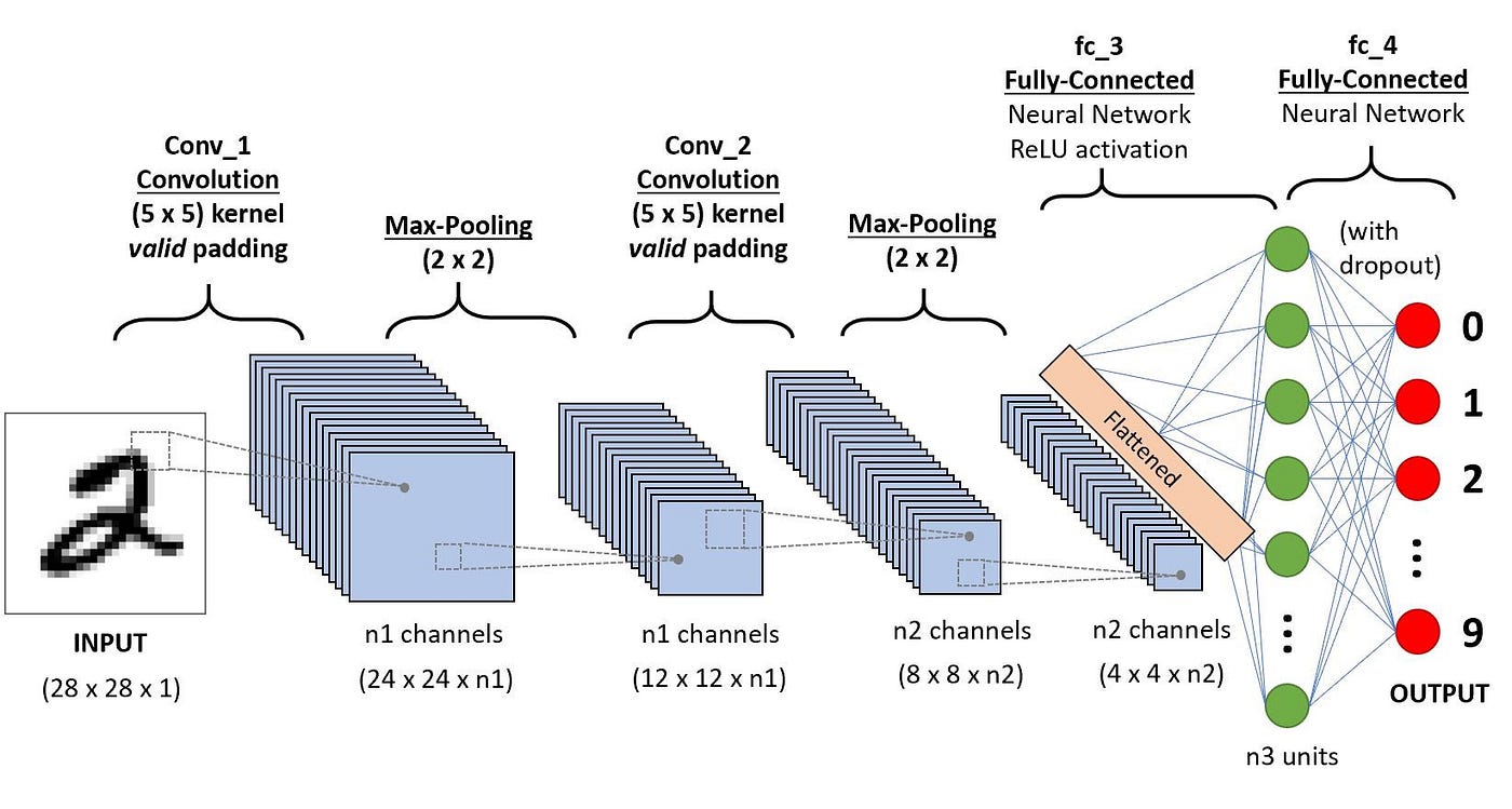
Just a reminder the CNN architecture has three very important parts:
- The convolution layer performs the function of convolving or sliding the filter over the input volume of images which are the source pixels (the kernel or filter can come in different matrices or tensors) depending on the images being greyscale or color channels(RGB) thereby computing the dot product of the filters and the source pixels. In other words the convolving operation is basically moving the entire filter across the entire image at each one time (number of strides).
2. Pooling layer performs the function of non-linear downsampling, what this is essentially saying is — it is progressively reducing the spatial size of the representation to reduce the amount of parameters and computation in the network. A huge benefit of this is to reducing the chances of the model overfitting. The most preferred method of pooling is Max-Pooling rather than Average-Pooling. Some of the reasons are because convolutions light up when they detect a particular feature in the region of an image and when downsampling , it makes sense to preserve the parts that were most activated.
3. And finally we have the fully connected layer or the dense layer which is just a linear stack of neural network layers that passes the output from the pooling layer to soft-max layer for the classification output
There is a major problem with CNN architectures being able to adapt to classifying videos, as we allayed to above CNNs are in no doubt near perfect algorithms in image recognition. But these images are fixed and can be cropped and rescaled to a fixed size, videos however have the time element attached(temporal attributes) to it which cannot be easily processed with a fixed-size architecture.
The Researchers resorted to treating each video as a bag of short, fixed-sized clips, and also knowing that each clip contains several frames in sequence in time, the connectivity of the network is extended in time dimension to learn spatial - temporal features (space-time features). A video with 30fps (frames per second) is halved to half a second which means we only consider 15 frames per half second.
A video compared to an image is a stack of frames, for example if you have a 200 x 200 resolution with RGB you would have 200 x 200 x 3 pixels, in each pixel it needs 8 bits to store the 0–255 values but a video would be a stack of these frames but for 1 second video you would have 30 images at 30 frames per second. The researchers in this study used 1 million YouTube videos in 487 classes .
The preprocessing of the data entailed the cropping of the videos to a fixed-size length and this is problematic because in sequence learning you won't be able to deal with variable length sequences, for example you won't be able to classify a 30 second video with the same ability as you would classify a 45 second video.
SPATIAL-TEMPORAL CONVOLUTION NEURAL NETWORKS
In order to solve the problem allayed to above they came up with Spatial-Temporal CNNs which is to take advantage of CNN's convolutional neural networks across different time scales.
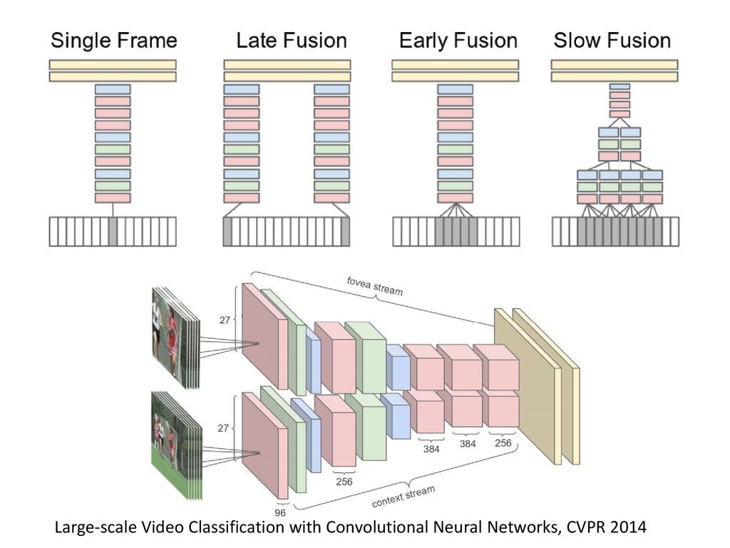
There are three broad network connectivity patterns used in this study, first one is Single Frame which just uses CNNs to extract image features from a single frame in the video.
Secondly, the Late Fusion which has very wide spaces between the frames used in the video to aggregate features and their experiment uses 15 frames in between the frames used in Late Fusion.The Late Fusion model places two separate single-frame networks with shared parameters a distance of 15 frames apart and then merges the two streams at the first fully connected layer. Therefore, neither single frame tower alone can detect any motion, but the first fully connected layer can compute global motion characteristics by comparing outputs of both towers.
Thirdly, Early Fusion collects a contiguous chunk of frames and processes it similar to the single frame model thereby combining information across an entire time window immediately on the pixel level. The early and direct connectivity to pixel data allows the network to precisely detect local motion direction and speed
Lastly, the Slow Fusion model takes interesting overlapping patches and processes them in separate architecture towers and then combines them later on thereby slowly fuses temporal information throughout the network such that higher layers get access to progressively more global information in both spatial and temporal dimensions. This is implemented by extending the connectivity of all convolutional layers in time and carrying out temporal convolutions in addition to spatial convolutions to compute activations. In the model they use, the first convolutional layer is extended to apply every filter of temporal extent T = 4 on an input clip of 10 frames through valid convolution with stride 2 and produces 4 responses in time. The second and third layers above iterate this process with filters of temporal extent T = 2 and stride 2. Thus, the third convolutional layer has access to information across all 10 input frames before being connected to the fully connected dense network layer.
MULTI-RESOLUTIONS CNNs
The multi-resolution model is used to reduce computation time since it will take weeks to train a large scale even on the fastest available GPUs. A solution was proposed: The proposed multi-resolution architecture aims to strike a compromise by having two separate streams of processing over two spatial resolutions called Context stream and Fovea stream. The context stream learns on low-resolution frames and the Fovea stream is a high resolution stream that only operates on the middle portion of the frame. In the second diagram above, on the top is the center crop from the original high resolution images and on the bottom is the downsized original image.
They were able to achieve 2–4x increase in runtime due to reduced input dimensionality. For example a 178 x 178 frame video clip :
a. Context stream — 89x89 downsized clip at half the original resolution
b. Fovea stream — 89x89 center crop of the original resolution. In this way, the the total input dimensionality is halved. This design takes advantage of the camera bias present in many online videos, since the object of interest often occupies the center region.
Since the input is only of half the spatial size as the full-frame models we discussed above, they take out the last pooling layer to ensure that both streams still terminate in a layer of size 7×7×256. The activations from both streams are concatenated and fed into the first fully connected layer with dense connections.
DATA AUGMENTATION AND PRE-PROCESSING
Data Augmentation was implemented to reduce the effects of overfitting, resizing and cropping of the frames is performed, in this instance to a 200 x 200 pixel, 170 x170 region is randomly sampled along with horizontal flipping of the frames 50% of the time and as a last step of pre-processing, they subtracted a constant value of 117 from the value of the pixels which is a approximate value of the mean of all pixels.
RESULTS OF THE STUDY
The Sports-1M dataset used has a hierarchical output space which tends to point to the fact that the model predicts the classes as related unlike normal unrelated classification outputs.
The dataset consists of 6 different types of bowling, 7 different types of American football and 23 types of billiards.
The model predicts a traversal along the tree and it is criticised based on the leaf and hierarchical nodes as well. So even if the prediction result gets to the bowling node and gets the type of bowling wrong it will receive less of a loss than if it lands on one of the American Football parent nodes.
The dataset has between 1000–3000 videos per class and 5% of the videos are annotated with more than one class, some noise also exist in the dataset because of weakly annotated videos — an example is labels based on tag prediction algorithm or uploader provided description and ultimately frame level variation. An example of Frame level variation takes an instance of a video labeled football, some of the frames might contain actual football being played or the scoreboard or the sky etc..
The training of the network happened over a period of one month, they were able to conclude that the multi-resolution network had a faster computational time than the full frame network. 5 clips per second for the full frame networks and 20 clips per second for the multi-resolution networks.To produce predictions for an entire video they randomly sampled 20 clips and present each clip individually to the network. Every clip is propagated through the network 4 times (with different crops and flips).

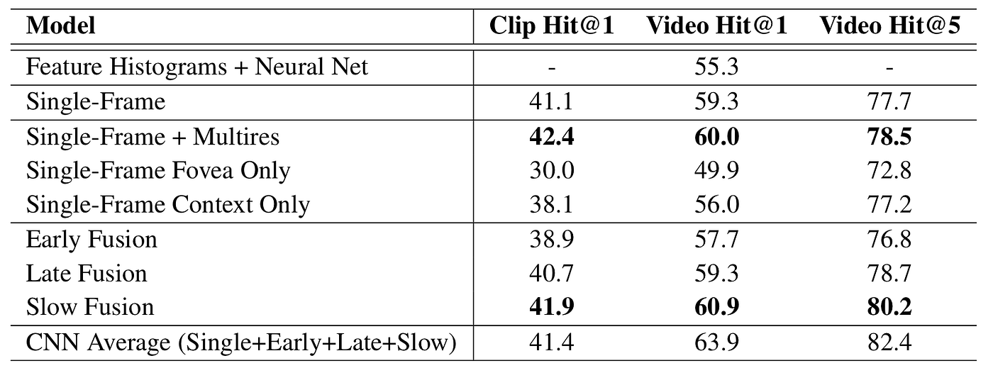
To produce video-level predictions they opted for the simplest approach of averaging individual clip predictions over the durations of each video. The table above shows the fraction of test samples that contain at least one ground truth label in the top k predictions with.
In conclusion, the researchers found that CNN architectures are capable of learning powerful features from weakly-labeled data that far surpass feature based methods in performance and that these benefits are surprisingly robust to details of the connectivity of the architectures in time as evidenced by the Slow Fusion model.
REFERENCES
- https://www.cvfoundation.org/openaccess/content_cvpr_2014/papers/Karpathy_Large-scale_Video_Classification_2014_CVPR_paper.pdf
atkinsetescashout1981.blogspot.com
Source: https://medium.com/analytics-vidhya/video-classification-using-cnns-db18bd2b7e72
0 Response to "How to Feed Cnn Network Video as Input"
Post a Comment